#data() # checking
data(Orange) # loadingData Structures in R
Important functions
ls() # list all the variables in the environment
rm(x) # can be used to remove specific var
#rm(list = ls()) # removes everything
Inbuild datasets in R
View(Orange) # opens a viewing window
head(Orange) # prints out first six rows on your console
Tree age circumference
1 1 118 30
2 1 484 58
3 1 664 87
4 1 1004 115
5 1 1231 120
6 1 1372 142tail(Orange) # prints out last six rows on your console Tree age circumference
30 5 484 49
31 5 664 81
32 5 1004 125
33 5 1231 142
34 5 1372 174
35 5 1582 177str(Orange) # tells you about the structure of the dataClasses 'nfnGroupedData', 'nfGroupedData', 'groupedData' and 'data.frame': 35 obs. of 3 variables:
$ Tree : Ord.factor w/ 5 levels "3"<"1"<"5"<"2"<..: 2 2 2 2 2 2 2 4 4 4 ...
$ age : num 118 484 664 1004 1231 ...
$ circumference: num 30 58 87 115 120 142 145 33 69 111 ...
- attr(*, "formula")=Class 'formula' language circumference ~ age | Tree
.. ..- attr(*, ".Environment")=<environment: R_EmptyEnv>
- attr(*, "labels")=List of 2
..$ x: chr "Time since December 31, 1968"
..$ y: chr "Trunk circumference"
- attr(*, "units")=List of 2
..$ x: chr "(days)"
..$ y: chr "(mm)"dim(Orange) # dimensions of the data - in terms of rows and columns[1] 35 3Data frames
A data frame is a rectangular collection of values, usually organized so that variables appear in the columns and observations appear in rows.
Creating a data frame
# Creating a new data frame that has 3 vectors of different types
dat.new <- data.frame(name = c("Anna", "Bob", "Chris"),
                    language = c("R", "C", "Java"),
                    year = c(4, 5, 9))

# View the dataframe
head(dat.new)
name language year
1 Anna R 4
2 Bob C 5
3 Chris Java 9Reading and writing a dataframe to a file
# This will add additional row names
write.csv(dat.new,file = "my_data.csv")
read.csv("my_data.csv") X name language year
1 1 Anna R 4
2 2 Bob C 5
3 3 Chris Java 9# To avoid adding row names to the data, use row.names=FALSE
write.csv(dat.new,file = "my_data.csv", row.names = FALSE)
read.csv("my_data.csv") # reads into the console name language year
1 Anna R 4
2 Bob C 5
3 Chris Java 9# To save the data into a variable:
dat.new2<- read.csv("my_data.csv")Working with data frames
dat.new2<- read.csv("my_data.csv")
# Note that you should have your entire path for the data under the quotes
# if your data is not saved in the working directory
# names of the data
names(dat.new2) [1] "name" "language" "year" # column names
colnames(dat.new2) [1] "name" "language" "year" # rownames
rownames(dat.new2)[1] "1" "2" "3"# type of data
class(dat.new2) [1] "data.frame"# structure of data
str(dat.new2) 'data.frame': 3 obs. of 3 variables:
$ name : chr "Anna" "Bob" "Chris"
$ language: chr "R" "C" "Java"
$ year : int 4 5 9Accessing values in a dataframe
# accessing a vector in the dataframe
dat.new2$name [1] "Anna" "Bob" "Chris"# accessing a second element of a vector in the dataframe
dat.new2$name[2] [1] "Bob"# accessing the language in the dataframe
dat.new2$language [1] "R" "C" "Java"# accessing a third element of a vector in the dataframe
dat.new2$language[3] [1] "Java"# Removing rows
dat.new2[-2,] name language year
1 Anna R 4
3 Chris Java 9# Removing columns
dat.new2[,-1] language year
1 R 4
2 C 5
3 Java 9# Appending to a data frame
dat.new3<- data.frame(name = c("Diego", "Evan", "Felicia", "George"), language = c("Python", "Perl", "C++","HTML"),
year = c(4, 5, 9,10))
# Binding by row
rbind(dat.new2,dat.new3) name language year
1 Anna R 4
2 Bob C 5
3 Chris Java 9
4 Diego Python 4
5 Evan Perl 5
6 Felicia C++ 9
7 George HTML 10newdata<-rbind(dat.new2,dat.new3)
# Binding by column
# cbind(dat.new2,dat.new3) # will give you error
## why this error? Because to bind by column, the number of rows should be equal
dat.new4<-dat.new3[-3,] # removing a row from 3rd data frame and adding to a new data frame
cbind(dat.new4,dat.new2) name language year name language year
1 Diego Python 4 Anna R 4
2 Evan Perl 5 Bob C 5
4 George HTML 10 Chris Java 9# Notice that R doesn't care about the content but the structure of data Subsetting dataframes
# The notation is nameofdata[row, column]
newdata[4,2][1] "Python"# accessing more than one value
newdata[1:4,] # gets you first four rows and all the columns name language year
1 Anna R 4
2 Bob C 5
3 Chris Java 9
4 Diego Python 4newdata[,1:2] # all the rows and first two columns name language
1 Anna R
2 Bob C
3 Chris Java
4 Diego Python
5 Evan Perl
6 Felicia C++
7 George HTML# Extracting specific information:
newdata[c(1,3),] # Gets you first and third row and all columns name language year
1 Anna R 4
3 Chris Java 9newdata[c(5,4),c(1,2)] # Guess name language
5 Evan Perl
4 Diego Python## Tip:
# Remember that the order of extraction matters.
## Accessing by name
newdata["name"] name
1 Anna
2 Bob
3 Chris
4 Diego
5 Evan
6 Felicia
7 Georgenewdata["year"] year
1 4
2 5
3 9
4 4
5 5
6 9
7 10## Operator
newdata$name[1] "Anna" "Bob" "Chris" "Diego" "Evan" "Felicia" "George" Matrices
In R, a matrix is a collection of elements of the same data type (numeric, character, or logical) arranged into a fixed number of rows and columns. A matrix is two-dimensional, since we are only working with rows and columns.
# Creating a new empty matrix
mat.example <- matrix(0, ncol=8, nrow=4)
# viewing the matrix
View(mat.example)
# class
class(mat.example) [1] "matrix" "array" # rows and columns
dim(mat.example) [1] 4 8# accessing column number
ncol(mat.example) [1] 8# accessing row numbers
nrow(mat.example) [1] 4Creating data using rnorm function
# Creating a new matrix with data:
# Using rnorm to generate 20 random numbers
mat.dat<-rnorm(20)
# Note that the random numbers will be different every time you run this code,
# Note check ?rnorm ?pnorm ?dnorm for more information on using probability distribution
mat.dat [1] -0.03753919 0.19505546 -0.40271567 0.39525381 1.21047045 1.45141048
[7] -1.98718050 -2.19437748 -1.59779674 -1.05152747 2.06239693 0.62811599
[13] 1.14914210 -0.63182229 0.44387661 0.21731383 -1.37358543 1.18468305
[19] 0.09138650 0.66010948# populating the matrix by row
mat.example2<-matrix(data = mat.dat, nrow = 4, ncol = 5, byrow = TRUE) Subsetting Matrices
# Subsetting rows and columns
mat.example2[2,4][1] -1.597797Lists in R
Lists are the R objects and contain elements of different types, For example a list can have numbers, characters, strings, vectors, matrix and another list inside it. A list can also have a function as one of its elements.
list_data<-list("Red","Green", c(21,34,22), TRUE, 52.53, 193.8)
list_data[[1]]
[1] "Red"
[[2]]
[1] "Green"
[[3]]
[1] 21 34 22
[[4]]
[1] TRUE
[[5]]
[1] 52.53
[[6]]
[1] 193.8list_data_new<-list(dat.new2, mat.example2)
list_data_new[[1]]
   name language year
1  Anna        R    4
2   Bob        C    5
3 Chris     Java    9
[[2]]
            [,1]       [,2]       [,3]       [,4]       [,5]
[1,] -0.03753919  0.1950555 -0.4027157  0.3952538  1.2104704
[2,]  1.45141048 -1.9871805 -2.1943775 -1.5977967 -1.0515275
[3,]  2.06239693  0.6281160  1.1491421 -0.6318223  0.4438766
[4,] 0.21731383 -1.3735854 1.1846831 0.0913865 0.6601095Subsetting lists
list_data[[3]][1] 21 34 22list_data_new[[2]] [,1] [,2] [,3] [,4] [,5]
[1,] -0.03753919 0.1950555 -0.4027157 0.3952538 1.2104704
[2,] 1.45141048 -1.9871805 -2.1943775 -1.5977967 -1.0515275
[3,] 2.06239693 0.6281160 1.1491421 -0.6318223 0.4438766
[4,] 0.21731383 -1.3735854 1.1846831 0.0913865 0.6601095Bonus activity - Plotting in R (using base R)
Base R can be used to create simple plots.
#--------Basic scatterplot

# Create data for plot
x<- seq(1,100, by=3)
y<- x/2

# Basic x and y plot
plot(x,y) 
# Add title
plot(x,y,main="Title of plot") 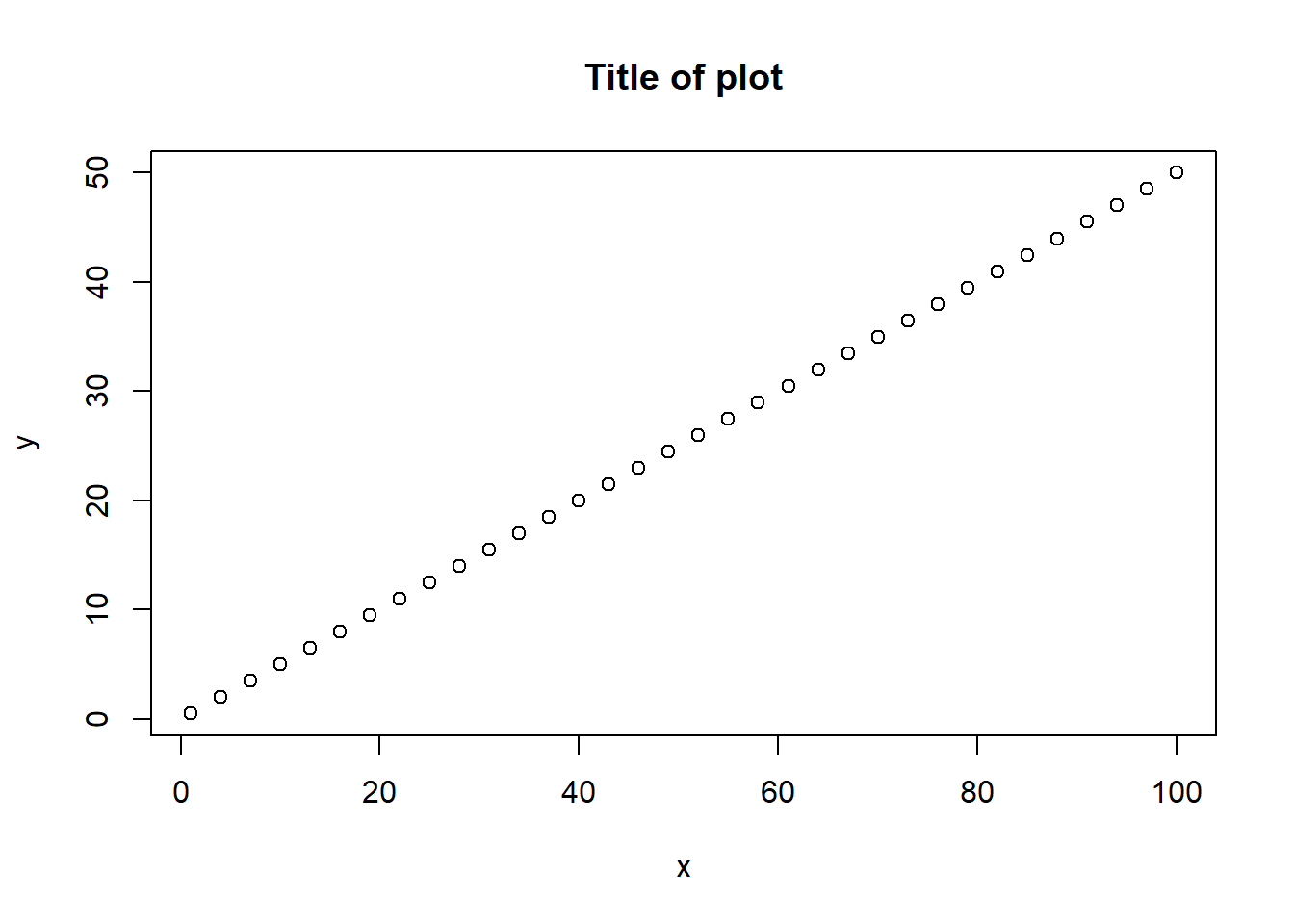
# Add x and y labels
plot(x,y,main="Title of plot",xlab = "This is x axis label",
     ylab="This is y label")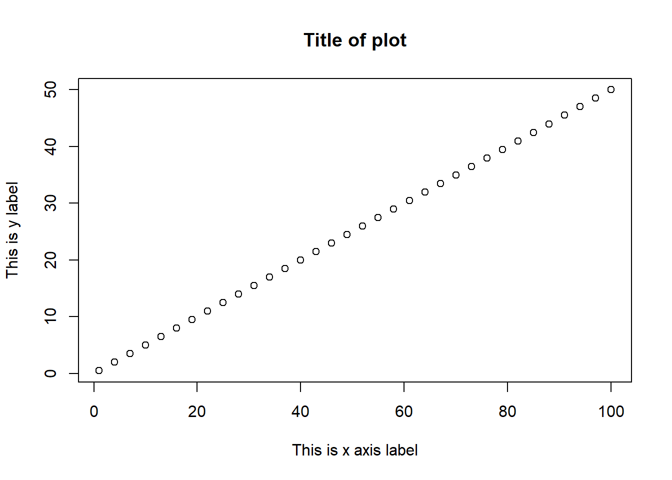
# Change color

plot(x,y,main="Title of plot",xlab = "This is x axis label",
     ylab="This is y label",col="blue")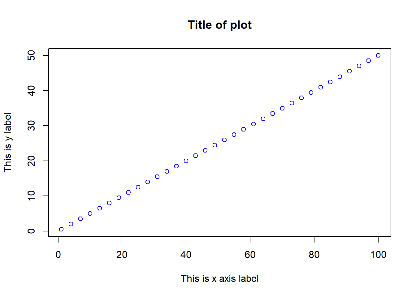
Histograms
# rnorm generates a vector of normally distributed random numbers.

x<-rnorm(1000, mean = 0, sd = 1)
hist(x)
hist(x, breaks = 10)
hist(x, breaks = 100)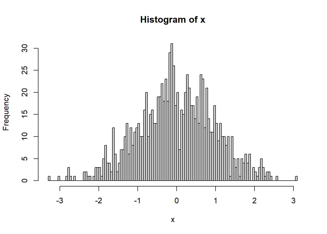
hist(x, breaks = 100, col = "orange", main = "This is title",
     xlab = "This is x axis", ylab = "This is y axis")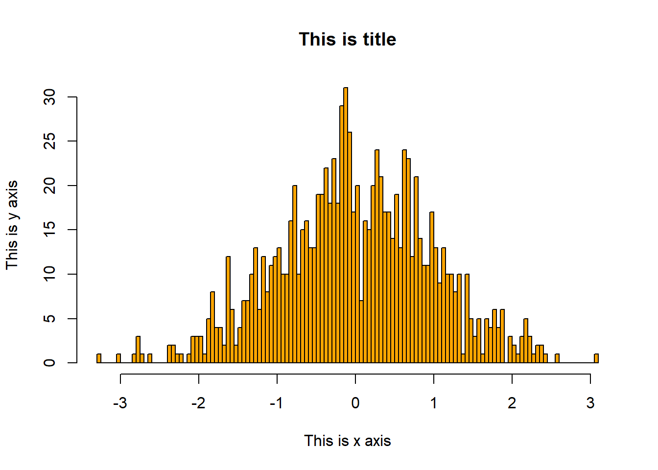
Questions from the workshop
Q1: How to sort dataframes?
# Use sort function to sort a vector
x<-c(1:10,8.5,7.6,2.5,1.3,2.4)
sort(x)
[1] 1.0 1.3 2.0 2.4 2.5 3.0 4.0 5.0 6.0 7.0 7.6 8.0 8.5 9.0 10.0# For sorting dataframes using the function order
newdata[order(newdata$year, decreasing = TRUE), ] name language year
7 George HTML 10
3 Chris Java 9
6 Felicia C++ 9
2 Bob C 5
5 Evan Perl 5
1 Anna R 4
4 Diego Python 4# Notice that the above function is used at the row position since we are sorting by row
# Another example:
newdata2<-data.frame(col1=c(31:40),col2=c(seq(1,30,by=3)))
newdata2 col1 col2
1 31 1
2 32 4
3 33 7
4 34 10
5 35 13
6 36 16
7 37 19
8 38 22
9 39 25
10 40 28newdata2[order(newdata2$col1, decreasing = TRUE),] col1 col2
10 40 28
9 39 25
8 38 22
7 37 19
6 36 16
5 35 13
4 34 10
3 33 7
2 32 4
1 31 1Q2: How to increase the number of rows displaying on console?
# Using the head command, where n is followed by number of rows

head(newdata2) # normally yields the first 6 rows
col1 col2
1 31 1
2 32 4
3 33 7
4 34 10
5 35 13
6 36 16head(newdata2,n=9)# would yield the first 9 rows col1 col2
1 31 1
2 32 4
3 33 7
4 34 10
5 35 13
6 36 16
7 37 19
8 38 22
9 39 25Q3: Can I use a graph in list?
# Answer: Not as an image but you can add a figure/graph as an object
# For example:
h1<-hist(rnorm(1000))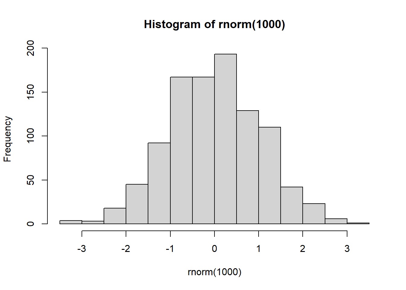
h2<-hist(rnorm(1000))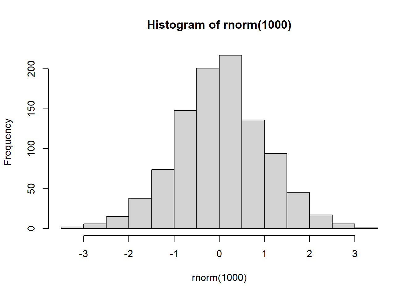
list.example<-list(h1,h2)
# The above example won't save the graph but the attributes
list.example
[[1]]
$breaks
[1] -3.5 -3.0 -2.5 -2.0 -1.5 -1.0 -0.5 0.0 0.5 1.0 1.5 2.0 2.5 3.0
$counts
[1] 3 10 11 45 92 157 175 197 142 109 39 18 2
$density
[1] 0.006 0.020 0.022 0.090 0.184 0.314 0.350 0.394 0.284 0.218 0.078 0.036
[13] 0.004
$mids
[1] -3.25 -2.75 -2.25 -1.75 -1.25 -0.75 -0.25 0.25 0.75 1.25 1.75 2.25
[13] 2.75
$xname
[1] "rnorm(1000)"
$equidist
[1] TRUE
attr(,"class")
[1] "histogram"
[[2]]
$breaks
[1] -3.0 -2.5 -2.0 -1.5 -1.0 -0.5 0.0 0.5 1.0 1.5 2.0 2.5 3.0 3.5
$counts
[1] 7 11 40 93 153 194 201 156 89 39 13 1 3
$density
[1] 0.014 0.022 0.080 0.186 0.306 0.388 0.402 0.312 0.178 0.078 0.026 0.002
[13] 0.006
$mids
[1] -2.75 -2.25 -1.75 -1.25 -0.75 -0.25 0.25 0.75 1.25 1.75 2.25 2.75
[13] 3.25
$xname
[1] "rnorm(1000)"
$equidist
[1] TRUE
attr(,"class")
[1] "histogram"# Using ggplot2 you can save the graph information as well
library(ggplot2)
df <- data.frame(x = rnorm(10), y = rnorm(10))
fig1 <- ggplot(df, aes(x, y)) + geom_point() + ggtitle("Graph 1")
fig2 <- ggplot(df, aes(x, y)) + geom_point() + ggtitle("Graph 2")
figlist <- list(fig1,fig2)
figlist[[1]]
[[2]]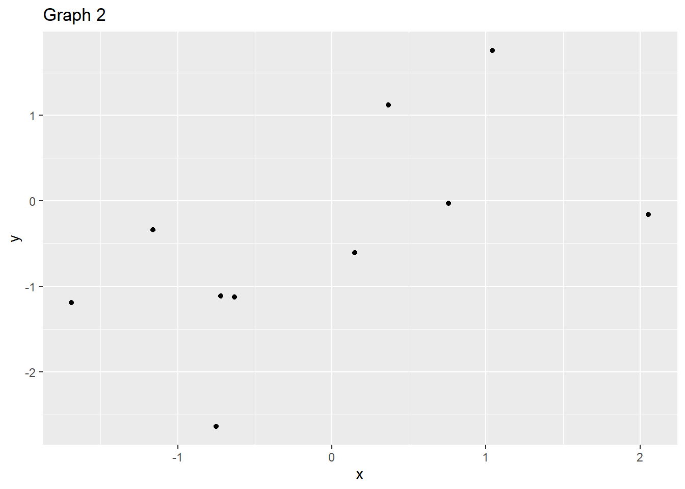
Q4: Difference between data.frame and data.table?
The stackoverflow post provided an excellent answer of the syntax differences between data frame and data table, so I highly encourage folks to read the information on this link along with the beginner’s FAQs for data.table here